There’s a specific kind of measurement problem worth naming precisely rather than dramatizing: this month we found that our model-routing agent was assigning a token budget to every unit of work, and that budget was noise in the strict sense. Fixing it meant improving a system that’s mostly right, not tearing one down.
(A quick note on scope: CloudZero has an existing post on AI cost optimization whose strategy #5 covers routing simple queries to Haiku-class models and reserving frontier models for hard reasoning. That’s a routing strategy. This post is about something different and downstream of it: once you’ve picked a tier, how do you compute a defensible token budget for the work, in code, from measured signals?)
We ran three blind, independent draws asking the same model to estimate token_ceiling for the same real units of work, and the per-unit standard deviation came back at 10–30% of the mean on four of six units. That’s wide enough to flip a unit from “within budget” to “over budget” and back again, with nothing changing but the roll of the dice. Every downstream decision (dispatch, warning thresholds, whether we tell an engineer their agent run is about to blow past its ceiling) was sitting on top of a number that couldn’t hold still.
We tried to prompt our way out of it twice. Naming concrete examples in the prompt failed to beat the baseline, and the comparison itself turned out to sit inside the noise. Naming an explicit multiplier was worse, unambiguously: on a 3-draw average every unit’s estimate went down, because the model shrank its base estimate before applying the multiplier (tuning/results/2026-08-22-pass7-blind-vs-chief-of-staff-actuals.md, iterations 3 and 5).
After two prompt rewrites failed to fix it, we stopped trying to word the request better and changed what we were asking the model for.
Six bounded signals instead of one free-hand integer
The fix was to stop asking the model for a number it’s bad at and start asking it for judgments it’s good at. Our schema already had a shape that didn’t show the noise problem: bounded 0–100 effectiveness/efficiency/difficulty scores, each with a one-clause reason. Those scores held steady across draws in a way the raw integers never managed.
So we moved the whole thing: the LLM now rates six bounded [0.0, 1.0] signals, and code computes the token ceiling.
| Signal | 0.0 → 1.0 means | v1.0.0 weight | Status |
|---|---|---|---|
| tool_call_volume | one content-only turn → many rounds of tool use | 1.0 | Shipped |
| content_volume | one-line change → hundreds of lines of new material | 1.0 | Shipped |
| cross_reference_load | standalone file → must stay faithful to several artifacts at once | 1.0 | Shipped |
| validation_loop_iterations | no validator → mandatory validate-then-fix loop | 0.0 | Tested, rejected (dilutes) |
| context_ingestion_volume | short prompt → large body to read first | 0.0 | Tested, rejected (dilutes) |
| investigative_uncertainty | every target known → open-ended search with dead ends | 0.0 | Tested twice, split, net rejected |
The distinctions are deliberately narrow. tool_call_volume counts how many calls a unit needs, while investigative_uncertainty rates how likely each of those calls is to be productive. cross_reference_load asks whether the output must stay consistent with other artifacts. context_ingestion_volume asks how much has to be read before any of that starts. Each pair sits close enough to look redundant, and each half catches something its neighbor misses. The rejected-signal results below are where that distinction earned its keep.
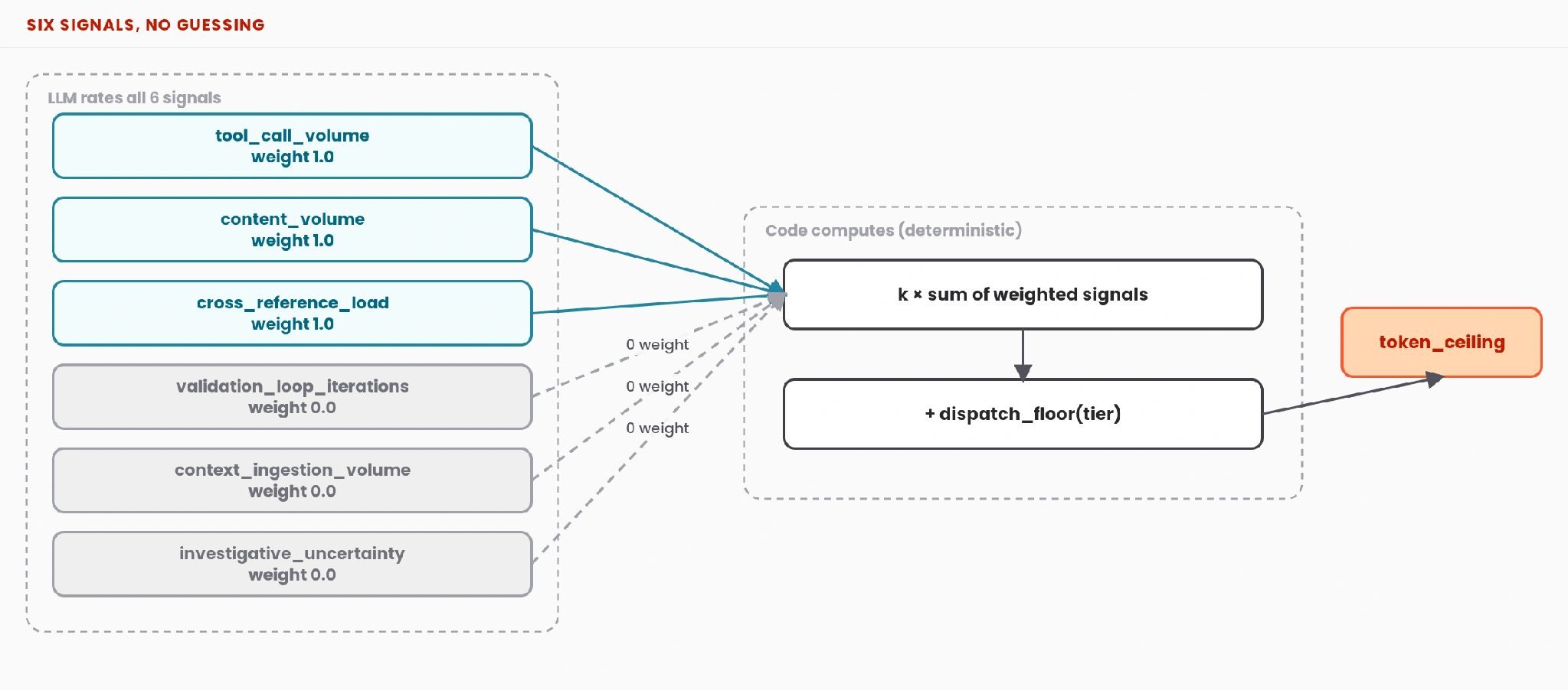
The LLM rates all six signals; code computes the token ceiling deterministically.
Report
Finance needs to prove AI’s return: CloudZero report
260 senior finance leaders (more than half CFOs) told us why the speed of seeing AI spend, not the size of it, separates who pulls ahead on AI from who gets burned.
Why did averaging cap what we could learn?
The v0 shape was:
| Symbol | Stands for |
|---|---|
| x₁, x₂, x₃ | tool_call_volume, content_volume, cross_reference_load — each ∈ [0.0, 1.0] |
| w₁, w₂, w₃ | their per-signal weights |
| t | tier (sonnet / opus / haiku) |
| F(t) | dispatch_floor(tier) |
| R(t) | real_work_span(tier) |
| s | real_work_scale |
| c | token_ceiling |
(This notation carries through the rest of the post.)
Walk through what that denominator actually forces. Take an equal split, w₁=w₂=w₃=⅓, against the same three signals the chart below uses — x₁=0.8, x₂=0.7, x₃=0.9:
Notice where 0.8 landed: between the smallest input (0.7) and the largest (0.9). That’s not a coincidence of these three numbers, rather it’s a property of every weighted average, for any nonnegative weights. Since each xᵢ ≤ max(x₁,x₂,x₃), the weighted sum w₁x₁+w₂x₂+w₃x₃ is at most max(x₁,x₂,x₃)·(w₁+w₂+w₃), and dividing by that same (w₁+w₂+w₃) leaves s ≤ max(x₁,x₂,x₃), always. No choice of weights escapes it.
Here’s why that’s a real problem and not a math curiosity. Genuinely hard work usually isn’t expensive because one dimension goes extreme; it’s expensive because several dimensions are moderately elevated at the same time. A lot of tool calls, and a lot of new content, and it has to stay consistent across several files. Three moderately-hard things happening together should cost more than any one of them alone. But s=0.8 above is still less than the single highest signal (0.9), and the average can never register “three things stacking” as worse than its single worst input, no matter how the weights are tuned (tuning/results/2026-08-22-weight-gradient-descent.md).
Compare that to the additive shape we ended up shipping: don’t divide.
Now three moderate signals stack past 1.0 instead of averaging back down into the pack. That’s exactly the behavior compound-hard work needs.
That gap isn’t academic once it hits real tokens. Run both scales through sonnet’s actual constants, F(t)=40,669 and R(t)=65,000: the averaged model gives c = 40,669 + 65,000·0.8 = 92,669 tokens; the additive model gives c = 40,669 + 65,000·1.422 ≈ 133,099 tokens. That’s a 40,430-token gap; the averaged formula under-predicts by 43.6% on exactly the “moderately hard on three fronts at once” shape of work that’s common in real compound tasks.
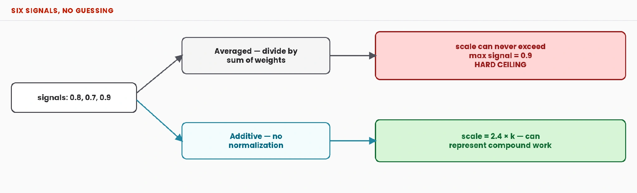
Averaged versus additive: the averaged scale can never exceed its own maximum signal.
Gradient descent found the answer by deleting a term
Dropping the normalization and gradient-descending the same three signals as a plain linear regression reached 94% training accuracy on an 18-row dataset, without adding a single new signal.
We then re-ran the fit using just one shared scalar instead of three separate weights — k(x₁ + x₂ + x₃) — with zero per-signal weight learning at all, and got identical accuracy. Turns out the three-weight fit was one effective degree of freedom wearing a three-parameter costume. It never actually learned “tool calls matter 1.3x more than content”; it learned one global scale correction (tuning/results/2026-08-22-additive-formula-and-signal-expansion.md).
So that’s what shipped:
The failure mode is dilution
Two of the six signals were rejected outright, and a third split; all three do correlate with real cost on their own. They failed because adding them made the combined signal worse.
The dominant failure mode for a candidate signal is dilution, not weak standalone correlation. That’s the most transferable thing this program produced.
A signal can be informative in isolation and still degrade the ensemble it’s added to:
| Signal | r alone | Sum’s correlation, before → after | Why it dilutes |
|---|---|---|---|
| validation_loop_iterations | 0.344 | 0.910 → 0.865 | Mean CV of 25.8% against 9.7–10.6% for the three shipped signals — 2.5x noisier. Correctly flags only 2 of 6 real training units; the other 4 are expensive for reasons it simply doesn’t see. |
| context_ingestion_volume | 0.766 | 0.910 → 0.880 | Tested on blind data — informative alone, still dilutes the sum. |
| investigative_uncertainty | — | Task 1: 0.910 → 0.980 (improves); Task 2: 0.994 → 0.936 (dilutes) | Tested twice, on two different held-out tasks, and the two runs disagreed. Net rejected for now, weight 0.0. |
investigative_uncertainty’s split leaves two live, untested hypotheses. The first is archetype-dependence: both held-out tasks so far were build/implementation units, and this signal was proposed as most load-bearing for finder/discovery work, which has never actually been tested. The second is plain sample-size noise: task 1 ran n=6 real units and task 2 ran n=4, small enough in both cases that one unit’s rating can swing the correlation.
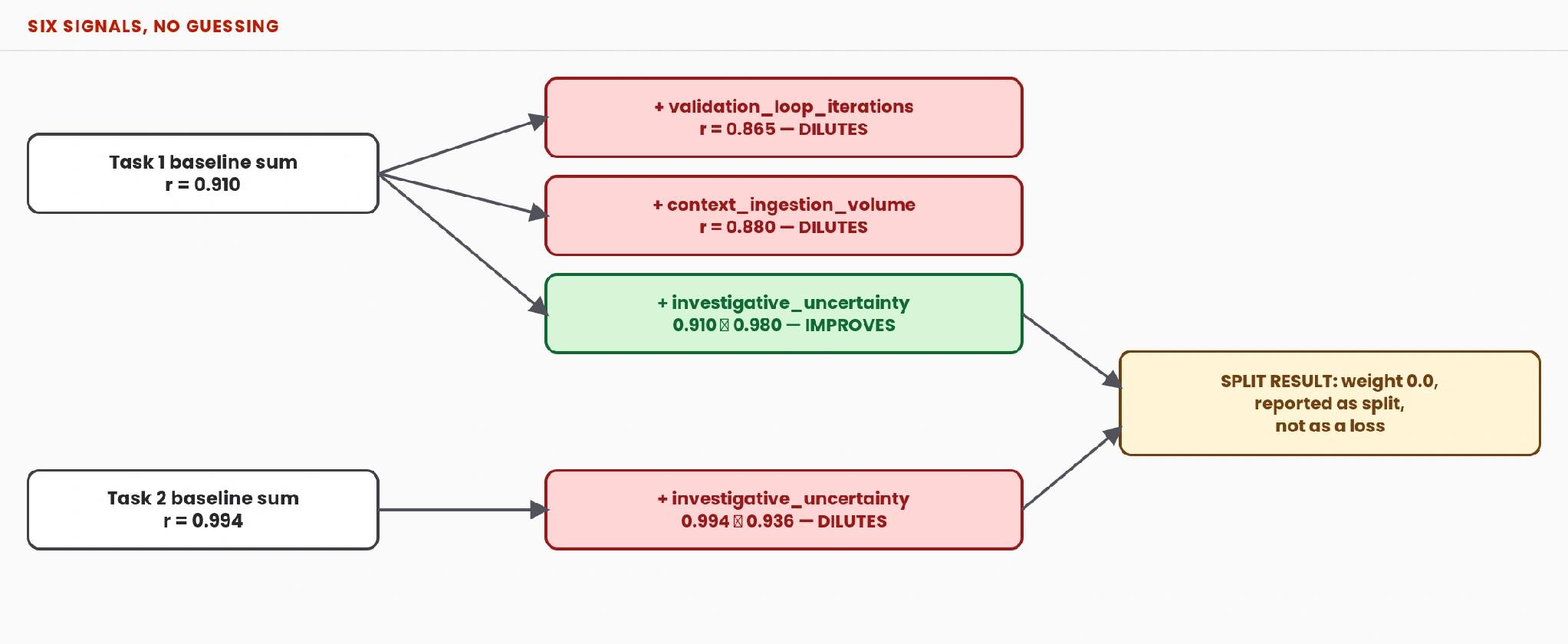
The dilution results: two signals dilute, one splits across two held-out tasks.
3/4 versus 0/4 on a fresh task
On a fresh held-out task; 4 real units, never used to fit k or any other constant, scored against the unchanged shipped constants; the additive model got accuracy_rate = 3/4 = 0.750 and the averaged model got 0/4 = 0.000. Same data, both models (tuning/results/2026-08-22-fresh-held-out-task-signal-and-formula-validation.md).
The asterisk that has to travel with that number: the averaged model’s 0/4 partly reflects a formula we had already mathematically proven incapable of doing better. Its capacity ceiling means no weight-tuning pass could have rescued it on this data. So the 0/4 measures the distance between a formula that can represent compound work and one that provably can’t.
The 3/4 has limits worth stating too: n=4, one task, one archetype. The single miss was the haiku tier, at a ratio of 1.041, barely over budget.
Where v1.0.0 actually stands
FORMULA_VERSION = “1.0.0” shipped on 2026-08-22, and the bar it clears is specific: every constant and default weight is backed by at least one real, disclosed experiment, with no first-principles guesses left waiting on data.
The constants as shipped:
| Tier | Dispatch floor | Real-work span | Additive total span (×k=0.5925) | Calibration |
|---|---|---|---|---|
| claude-sonnet-5 | 40,669 | 65,000 | 38,513 | Measured — n=4 real dispatches |
| claude-opus-4-8 | 38,260 | 61,150 | 36,231 | Placeholder — floor-ratio scaled from sonnet; n=2 real dispatches informed only the floor |
| claude-haiku-4-5 | 25,664 | 41,018 | 24,303 | Placeholder — floor-ratio scaled from sonnet; zero real per-unit dispatches |
(Only sonnet’s 65,000 span and the three dispatch floors are hard-coded in the module; the opus and haiku spans and all three additive spans are computed here from REAL_WORK_SPAN = 65_000 * floor_ratio and ADDITIVE_TOTAL_SPAN = span * 0.5925, not restated verbatim from the source.)
Sonnet’s 65,000 span is the best-calibrated number in the module: fit to 4 real sonnet dispatches from one real build (56,932 / 76,292 / 99,532 / 104,219 actual tokens, each net of the 40,669 zero-tool floor). Backing out the implied scale per unit reproduces 0.25, 0.55, 0.91, 0.98. A tight fit, though drawn from that single build.
None of this is finished. Each row names a current limitation.
| # | Gap | Why it’s ranked here |
|---|---|---|
| 1 | Haiku-tier calibration | The single weakest link. REAL_WORK_SPAN[“claude-haiku-4-5”] has never been independently measured (it’s floor-ratio scaled), and haiku was the one miss on the fresh task. Even the near-zero-work anchor needed real multi-file search to find its own edit. Fix: dispatch real haiku builds across a spread of work scales. |
| 2 | investigative_uncertainty’s split | Unresolved, not settled. Needs a third held-out task with an actual finder/discovery unit, ideally 6+ real units. |
| 3 | k = 0.5925 has one confirmation | Real and non-circular, but resting on a single held-out task at n=4 (see the section above for what that one miss was). |
| 4 | Two signals never tested at all | shared_file_blast_radius and voice_or_precision_consistency_requirement, both reasoned from real task shapes and never wired in. Not rejected, just untouched. |
| 5 | Two unreconciled floor measurements | Shipped floors (40,669 / 38,260 / 25,664) vs. a second harness measurement (42,512 / 42,416 / 32,653). Probably the same mechanism with n=1-per-tier noise. Never reconciled. |
Consider this an open invitation: if you’re already dispatching real sub-agent work and can spare a few units, here’s how to help close one of these. Run model-right-sizer-holdout-tuning against a haiku-tier task to take a swing at gap #1, or model-right-sizer-signal-validation against a genuine finder/discovery task for gap #2.
Six signals, no guessing. That’s the whole idea. Six numbers you can point to beat one guess you can’t.